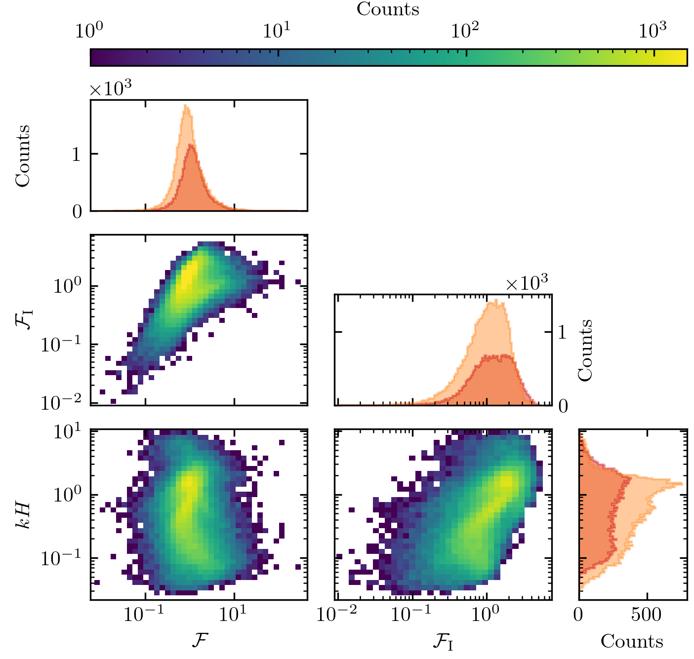
Figure 10 – Online Resource

import os
import sys
import numpy as np
import matplotlib.pyplot as plt
from matplotlib.colors import LogNorm
sys.path.append('../../')
import python_codes.theme as theme
from python_codes.plot_functions import make_nice_histogram

theme.load_style()

# paths
path_savefig = '../../Paper/Figures'
path_outputdata = '../../static/data/processed_data/'

# Loading data
Data = np.load(os.path.join(path_outputdata, 'Data_final.npy'), allow_pickle=True).item()
Stations = ['South_Namib_Station', 'Deep_Sea_Station']

numbers = {key: np.concatenate([Data[station][key] for station in Stations]) for key in ('Froude', 'kH', 'kLB')}
mask = ~np.isnan(numbers['Froude'])
ad_hoc_quantity = np.concatenate([Data[station]['U_star_era'] for station in Stations])

# Figure properties
couples = [('Froude', 'kLB'), ('Froude', 'kH'), ('kLB', 'kH')]
lims = {'Froude': (5.8e-3, 450), 'kLB': (0.009, 7.5), 'kH': (2.2e-2, 10.8)}
# ax_labels = {'kH': r'$kH$', 'Froude': r'$\mathcal{F} =  U/\sqrt{(\Delta\rho/\rho) g H}$',
# 'kLB': r'$\mathcal{F}_{\textup{I}} =  kU/N$'}
ax_labels = {'kH': r'$kH$', 'Froude': r'$\mathcal{F}$',
             'kLB': r'$\mathcal{F}_{\textup{I}}$'}
norm = LogNorm(vmin=1, vmax=1.5e3)

# #### Figure
fig, axarr = plt.subplots(4, 3, figsize=(theme.fig_width, 0.95*theme.fig_width),
                          # constrained_layout=True,
                          gridspec_kw={'height_ratios': [0.2, 1.3, 2, 2],
                                       'width_ratios': [2, 2, 1]})
# Plotting density diagrams
ax_list = [axarr[2, 0], axarr[3, 0], axarr[3, 1]]
for j, (ax, (var1, var2)) in enumerate(zip(ax_list, couples)):
    ax.set_xscale('log')
    ax.set_yscale('log')
    #
    x_var, y_var = numbers[var1][mask], numbers[var2][mask]
    xlabel = ax_labels[var1]
    ylabel = ax_labels[var2] if j == 0 else None
    #
    bin1 = np.logspace(np.floor(np.log10(numbers[var1][mask].min())), np.ceil(np.log10(numbers[var1][mask].max())), 50)
    bin2 = np.logspace(np.floor(np.log10(numbers[var2][mask].min())), np.ceil(np.log10(numbers[var2][mask].max())), 50)
    # #### binning data
    counts, x_edge, y_edge = np.histogram2d(x_var, y_var, bins=[bin1, bin2])
    # plotting histogramm
    a = ax.pcolormesh(x_edge, y_edge, counts.T, snap=True, norm=norm)
    #
    ax.set_xlim(lims[var1])
    ax.set_ylim(lims[var2])
    if j in [1, 2]:
        ax.set_xlabel(ax_labels[var1])
    else:
        ax.set_xticklabels([])
    if j in [0, 1]:
        ax.set_ylabel(ax_labels[var2])
    else:
        ax.set_yticklabels([])

# #### Plotting marginal distributions
for i, (ax, var) in enumerate(zip([axarr[1, 0], axarr[2, 1], axarr[3, 2]], ['Froude', 'kLB', 'kH'])):
    orientation = 'vertical' if i < 2 else 'horizontal'
    make_nice_histogram(Data['South_Namib_Station'][var], 150, ax, alpha=0.4,
                        density=False, scale_bins='log', orientation=orientation,
                        color=theme.color_Era5Land_sub)
    make_nice_histogram(Data['Deep_Sea_Station'][var], 150, ax, alpha=0.4,
                        density=False, scale_bins='log', orientation=orientation,
                        color=theme.color_Era5Land)
    if i == 2:
        ax.set_ylim(lims[var])
        ax.set_yticklabels([])
        ax.set_xlabel('Counts')
        # ax.ticklabel_format(style='sci', axis='x', scilimits=(0, 0))
    elif i == 0:
        ax.set_ylabel('Counts')
        ax.set_xticklabels([])
        ax.set_xlim(lims[var])
        ax.ticklabel_format(style='sci', axis='y', scilimits=(0, 0))
    elif i == 1:
        ax.set_xticklabels([])
        ax.set_ylabel('Counts')
        ax.set_xlim(lims[var])
        ax.yaxis.tick_right()
        ax.yaxis.set_label_position('right')
        ax.yaxis.set_ticks_position('both')
        ax.ticklabel_format(style='sci', axis='y', scilimits=(0, 0))

# remove the underlying axes for cb
gs = axarr[0, 0].get_gridspec()
for ax in axarr[0, :]:
    ax.remove()
cax = fig.add_subplot(gs[0, :])
#
cb = fig.colorbar(a, cax=cax, label='Counts', orientation='horizontal')
cb.ax.xaxis.set_ticks_position('top')
cb.ax.xaxis.set_label_position('top')
#
# removing unused axes
axarr[1, 1].remove()
axarr[1, 2].remove()
axarr[2, -1].remove()
#
plt.subplots_adjust(bottom=0.09, top=0.91, left=0.13, right=0.99, hspace=0.2, wspace=0.15)
#
# Adjusting final ax positions
# cb
pos = cax.get_position()
cb_h = pos.height
pos.y0 = 0.9
pos.y1 = pos.y0 + cb_h
cax.set_position(pos)
# distrib 2
box1 = axarr[1, 0].get_position()
pos = axarr[2, 1].get_position()
pos.y1 = pos.y0 + box1.height
axarr[2, 1].set_position(pos)

fig.align_labels()
plt.savefig(os.path.join(path_savefig, 'Figure10_supp.pdf'))
plt.show()