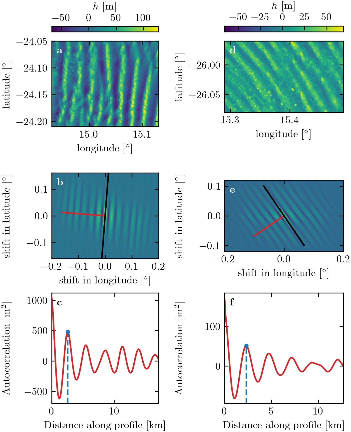
Figure 4 – Online Resource

import os
import sys
import numpy as np
import matplotlib.pyplot as plt
import matplotlib.transforms as mtransforms
from types import SimpleNamespace
sys.path.append('../../')
import python_codes.theme as theme
from python_codes.general import cosd, sind

theme.load_style()

# paths
path_savefig = '../../Paper/Figures'
path_outputdata = '../../static/data/processed_data/'

Data_DEM = np.load(os.path.join(path_outputdata, 'Data_DEM.npy'),
                   allow_pickle=True).item()

labels = [r'\textbf{a}', r'\textbf{b}',  r'\textbf{c}', r'\textbf{d}',
          r'\textbf{e}', r'\textbf{f}']

fig, axrr = plt.subplots(3, 2, figsize=(theme.fig_width, 0.75*theme.fig_height_max),
                         constrained_layout=True, gridspec_kw={'width_ratios': (0.9, 1)})
for i, station in enumerate(Data_DEM.keys()):
    # loading into namespace from data dictionnary to shorten call
    n = SimpleNamespace(**Data_DEM[station])
    # ax0: Topo
    cs = axrr[0, i].contourf(n.lon, n.lat, n.topo, levels=50)
    for c in cs.collections:
        c.set_edgecolor("face")
        c.set_rasterized(True)
    if i == 0:
        ticks = [-50, 0, 50, 100]
    else:
        ticks = [-50, -25, 0, 25, 50]
    cb = fig.colorbar(cs, ax=axrr[0, i], label='$h$~[m]', location='top', ticks=ticks)
    cb.ax.locator_params(nbins=8)
    axrr[0, i].set_xlabel(r'longitude [$^{\circ}$]')
    axrr[0, i].set_ylabel(r'latitude [$^{\circ}$]')
    axrr[0, i].set_aspect('equal')
    #
    # ax1: Autocorrelation map
    x = list(-(n.lon - n.lon[0])[:: -1]) + list((n.lon - n.lon[0])[1:])
    y = list(-(n.lat - n.lat[0])[:: -1]) + list((n.lat - n.lat[0])[1:])
    cs = axrr[1, i].contourf(x, y, n.C, levels=50)
    for c in cs.collections:
        c.set_edgecolor("face")
        c.set_rasterized(True)
    #
    axrr[1, i].plot([x[n.p0[0]], x[int(round(n.p1[0]))]], [y[n.p0[1]], y[int(round(n.p1[1]))]], color='tab:red', label='profile for wavelength calculation')
    p11 = n.p0 + np.array([cosd(n.orientation), sind(n.orientation)])*min(n.topo.shape)
    p12 = n.p0 - np.array([cosd(n.orientation), sind(n.orientation)])*min(n.topo.shape)
    axrr[1, i].plot([x[int(round(p11[0]))], x[int(round(p12[0]))]], [y[int(round(p11[1]))], y[int(round(p12[1]))]], color='k', label='n.orientation')
    axrr[1, i].set_xlabel(r'shift in longitude [$^{\circ}$]')
    axrr[1, i].set_ylabel(r'shift in latitude [$^{\circ}$]')
    axrr[1, i].set_aspect('equal')
    #
    # ax2: Autocorrelation profile
    mytrans = axrr[2, i].transData + axrr[2, i].transAxes.inverted()
    #
    x_transect = np.arange(n.transect.size)*n.km_step
    axrr[2, i].plot(x_transect, n.transect, color='tab:red')
    axrr[2, i].plot(x_transect[n.wavelength_indx], n.transect[n.wavelength_indx], color='tab:blue', marker='.')
    lims = axrr[2, i].get_ylim()
    axrr[2, i].vlines(x_transect[n.wavelength_indx], lims[0], n.transect[n.wavelength_indx], color='tab:blue', linestyle='--')
    axrr[2, i].set_xlabel('Distance along profile [km]')
    axrr[2, i].set_ylabel('Autocorrelation~[m$^{2}$]')
    axrr[2, i].set_xlim(0, x_transect.max())
    axrr[2, i].set_ylim(lims)
    #

trans = mtransforms.ScaledTranslation(5/72, -5/72, fig.dpi_scale_trans)
for i, (label, ax) in enumerate(zip(labels, axrr.T.flatten())):
    if i in [0, 1, 3, 4]:
        color = 'w'
    else:
        color = 'k'
    ax.text(0.0, 1.0, label, transform=ax.transAxes + trans, va='top', color=color)


fig.align_ylabels()
plt.savefig(os.path.join(path_savefig, 'Figure4_supp.pdf'), dpi=600)
plt.show()