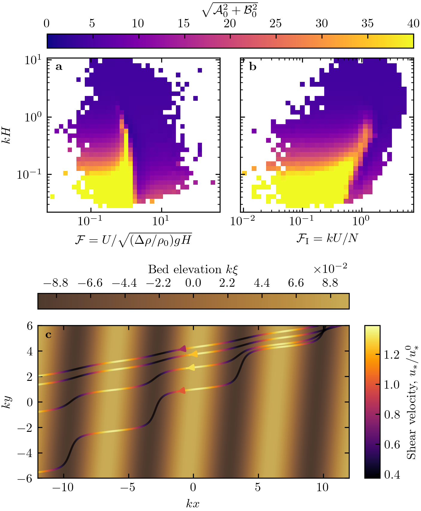
Figure 13 – Online Resource

import os
import sys
import numpy as np
import matplotlib.pyplot as plt
sys.path.append('../../')
import python_codes.theme as theme
from python_codes.general import cosd, sind
from python_codes.plot_functions import plot_regime_diagram
from python_codes.linear_theory import Cisaillement_basal_rotated_wind


def topo(x, y, alpha, k, xi):
    return xi*np.cos(k*(cosd(alpha)*x + sind(alpha)*y))


# Loading figure theme
theme.load_style()

# paths
path_savefig = '../../Paper/Figures'
path_outputdata = '../../static/data/processed_data/'

# ## regime diagram properties
# data
Stations = ['South_Namib_Station', 'Deep_Sea_Station']
Data = np.load(os.path.join(path_outputdata, 'Data_final.npy'), allow_pickle=True).item()
numbers = {key: np.concatenate([Data[station][key] for station in Stations]) for key in ('Froude', 'kH', 'kLB')}

# Time series hydrodynamic coefficients
Hydro_coeffs_time = np.load(os.path.join(path_outputdata, 'time_series_hydro_coeffs.npy'), allow_pickle=True).item()
modulus = np.linalg.norm(np.concatenate([Hydro_coeffs_time[station] for station in Stations], axis=1), axis=0)

#
couples = [('Froude', 'kH'), ('kLB', 'kH')]
labels = [r'\textbf{a}', r'\textbf{b}', r'\textbf{c}']
#
ax_labels = {'Froude': r'$\mathcal{F} =  U/\sqrt{(\Delta\rho/\rho_{0}) g H}$', 'kH': '$k H$', 'kLB': r'$\mathcal{F}_{\textup{I}} = k U/N$'}
lims = {'Froude': (5.8e-3, 450), 'kLB': (0.009, 7.5), 'kH': (2.2e-2, 10.8)}
#
regime_line_color = 'tab:blue'
cbar_labels = [r'$\delta_{\theta}$ [deg.]', r'$\delta_{u}$']

mask = ~np.isnan(numbers['Froude'])

# ## streamline parameters
station = Stations[1]
Data_DEM = np.load(os.path.join(path_outputdata, 'Data_DEM.npy'), allow_pickle=True).item()[station]

#
alpha = Data_DEM['orientation'] - 90  # dune orientation, degrees
k = 1  # non dimensional wavenumber
AR = 0.1
B0 = 2
skip = (slice(None, None, 50), slice(None, None, 50))
#
# horizontal space
x = np.linspace(-12, 12, 1000)
y = np.linspace(-6, 6, 1000)
X, Y = np.meshgrid(x, y)


# #### Figure
fig = plt.figure(figsize=(theme.fig_width, 0.74*theme.fig_height_max), constrained_layout=True)
# ## regime diagrams
gs = fig.add_gridspec(2, 1, height_ratios=[1.63, 1])
gs.update(hspace=0.1025)
gs_top = gs[0].subgridspec(1, 2)
axarr = []
for i, (var1, var2) in enumerate(couples):
    axarr.append(fig.add_subplot(gs_top[i]))
    vars = [numbers[var1][mask], numbers[var2][mask]]
    cmap = 'viridis'
    lims_list = [lims[var1], lims[var2]]
    xlabel = ax_labels[var1]
    ylabel = ax_labels[var2] if i == 0 else None
    #
    bin1 = np.logspace(np.floor(np.log10(numbers[var1][mask].min())), np.ceil(np.log10(numbers[var1][mask].max())), 50)
    bin2 = np.logspace(np.floor(np.log10(numbers[var2][mask].min())), np.ceil(np.log10(numbers[var2][mask].max())), 50)
    bins = [bin1, bin2]
    a = plot_regime_diagram(axarr[-1], modulus[mask], vars, lims_list, xlabel, ylabel, bins=bins, vmin=0, vmax=40, cmap='plasma', type='binned')
    axarr[-1].text(0.05, 0.92, labels[i], transform=axarr[-1].transAxes)

# #### colorbar
cb = fig.colorbar(a, ax=axarr, location='top', aspect=26,
                  label=r'$\sqrt{\mathcal{A}_{0}^{2} + \mathcal{B}_{0}^{2}}$')

# ## Examples
ax = fig.add_subplot(gs[1])
ax.set_xlabel('$kx$')
ax.set_ylabel('$ky$')
# ax.set_aspect('equal')
ax.text(0.025, 0.92, labels[2], transform=ax.transAxes)
#
cnt = ax.contourf(x, y, topo(X, Y, alpha, k, AR), levels=100, vmin=-(AR + 0.06),
                  vmax=AR + 0.02, zorder=-5, cmap=theme.cmap_topo)
for c in cnt.collections:
    c.set_edgecolor("face")
    c.set_rasterized(True)

# # #### Parameters
modulus = np.linalg.norm(Hydro_coeffs_time[station], axis=0)
indexes_tp = np.arange(Data[station]['kH'].size)
mask1 = (Data[station]['kH'] > 0.7) & (Data[station]['Froude'] > 0.6) & (modulus < 10)
mask2 = (Data[station]['kH'] > 0.7) & (Data[station]['Froude'] < 0.3) & (modulus < 10)
mask3 = (Data[station]['kH'] < 0.5) & (Data[station]['Froude'] > 0.6) & (modulus < 10)
mask4 = (Data[station]['kH'] < 0.5) & (Data[station]['Froude'] < 0.3) & (modulus < 10)

indexes = [2808, 35785, 6231, 11308]
#
for i, (m, A0, B0) in enumerate(sorted(zip(modulus[indexes], Hydro_coeffs_time[station][0][indexes], Hydro_coeffs_time[station][1][indexes]))):
    # print(Data[station]['time'][indexes[i]], Data[station]['kH'][indexes[i]], Data[station]['Froude'][indexes[i]], Data[station]['kLB'][indexes[i]], A0, B0, np.sqrt(A0**2 + B0**2))
    TAU = Cisaillement_basal_rotated_wind(X, Y, alpha, A0, B0, AR, 190)
    ustar = np.sqrt(np.linalg.norm(np.array(TAU), axis=0))
    theta = np.arctan2(TAU[1], TAU[0])
    # ax.quiver(X[skip], Y[skip], TAU[0][skip], TAU[1][skip], color='grey')
    # strm = ax.streamplot(X, Y, TAU[0], TAU[1], color=np.sqrt(TAU[0]**2 + TAU[1]**2), cmap='inferno', density=50, start_points=[[4, 5-0.5*i]])
    strm = ax.streamplot(X, Y, ustar*np.cos(theta), ustar*np.sin(theta),
                         color=ustar, cmap='inferno', density=50, start_points=[[4, 5-0.5*i]])
#
cb = fig.colorbar(cnt, label=r'Bed elevation $k \xi$', ax=ax, location='top', pad=0.08)
cb.formatter.set_powerlimits((0, 0))
cb.update_ticks()
cb = fig.colorbar(strm.lines, label=r'Shear velocity, $u_{*}/u_{*}^{0}$', ax=ax, location='right', aspect=10)

plt.savefig(os.path.join(path_savefig, 'Figure13_supp.pdf'), dpi=400)
plt.show()