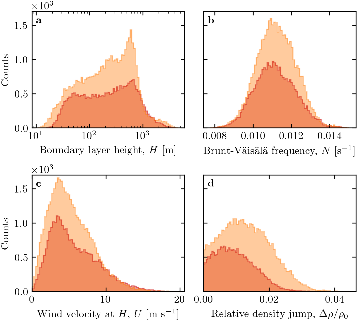
Figure 9 – Online Resource

import os
import sys
import numpy as np
import matplotlib.pyplot as plt
import matplotlib.transforms as mtransforms
sys.path.append('../../')
import python_codes.theme as theme
from python_codes.meteo_analysis import mu
from python_codes.plot_functions import make_nice_histogram


# Loading figure theme
theme.load_style()

# paths
path_savefig = '../../Paper/Figures'
path_outputdata = '../../static/data/processed_data/'

# ##### Loading meteo data
Data = np.load(os.path.join(path_outputdata, 'Data_final.npy'), allow_pickle=True).item()

# ## histograms parameters
Stations = ['South_Namib_Station', 'Deep_Sea_Station']
g = 9.81  # [m/s2] gravitational constant
z0_era = 1e-3  # [m] hydrodynamic roughness
#
labels = [r'\textbf{a}', r'\textbf{b}', r'\textbf{c}', r'\textbf{d}']
nbins = 80

# #### Figure
fig, axarr = plt.subplots(2, 2, figsize=(theme.fig_width, 0.9*theme.fig_width),
                          constrained_layout=True, sharey=True)

colors = [theme.color_Era5Land_sub, theme.color_Era5Land]
for station, color in zip(Stations, colors):
    make_nice_histogram(Data[station]['Boundary layer height'], nbins, axarr[0, 0],
                        alpha=0.4, label=' '.join(station.split('_')[:-1]),
                        density=False, scale_bins='log', color=color)
    #
    N = np.sqrt(g*Data[station]['gradient_free_atm']/Data[station]['theta_ground'])
    make_nice_histogram(N, nbins, axarr[0, 1], alpha=0.4, label=' '.join(station.split('_')[:-1]),
                        density=False, color=color)
    #
    U_H = Data[station]['U_star_era']*mu(Data[station]['Boundary layer height'], z0_era)
    make_nice_histogram(U_H, nbins, axarr[1, 0], alpha=0.4, label=' '.join(station.split('_')[:-1]),
                        density=False, color=color)
    #
    make_nice_histogram(Data[station]['delta_theta']/Data[station]['theta_ground'],
                        nbins, axarr[1, 1], alpha=0.4, label=' '.join(station.split('_')[:-1]),
                        density=False, color=color)


axarr[1, 0].set_xlim(left=0)
axarr[1, 1].set_xlim(left=0)
#
axarr[0, 0].set_xlabel(r'Boundary layer height, $H~[\textup{m}]$')
axarr[0, 1].set_xlabel(r'Brunt-Väisälä frequency, $N~[\textup{s}^{-1}]$')
axarr[1, 0].set_xlabel(r'Wind velocity at $H$, $U~[\textup{m}~\textup{s}^{-1}]$')
axarr[1, 1].set_xlabel(r'Relative density jump, $\Delta\rho/\rho_{0}$')
#

trans = mtransforms.ScaledTranslation(4/72, -4/72, fig.dpi_scale_trans)
for i, (ax, label) in enumerate(zip(axarr.flatten(), labels)):
    ax.set_ylim(0, 1700)
    ax.text(0.0, 1.0, label, transform=ax.transAxes + trans, va='top')
    ax.ticklabel_format(style='sci', axis='y', scilimits=(0, 0))
    if i not in [1, 3]:
        ax.set_ylabel('Counts')

fig.align_labels()
plt.savefig(os.path.join(path_savefig, 'Figure9_supp.pdf'))
plt.show()